angular and tangential velocity in circular motion
Angular and tangential velocity in circular motion
First, we need to clarify the notations.
We have a tangential velocity vector, \[\vec{v}\], representing how the position of an object changes with time. It tells you both how fast the object is moving and in which direction. It is comprised of the magnitude and directional component, i.e. \[\vec{v}=v_{\theta}\cdot\hat{\theta}\]. We refer to the tangential velocity vector when we want to include the full vector, i.e. with both magnitude and direction that is always tangent to the circle.
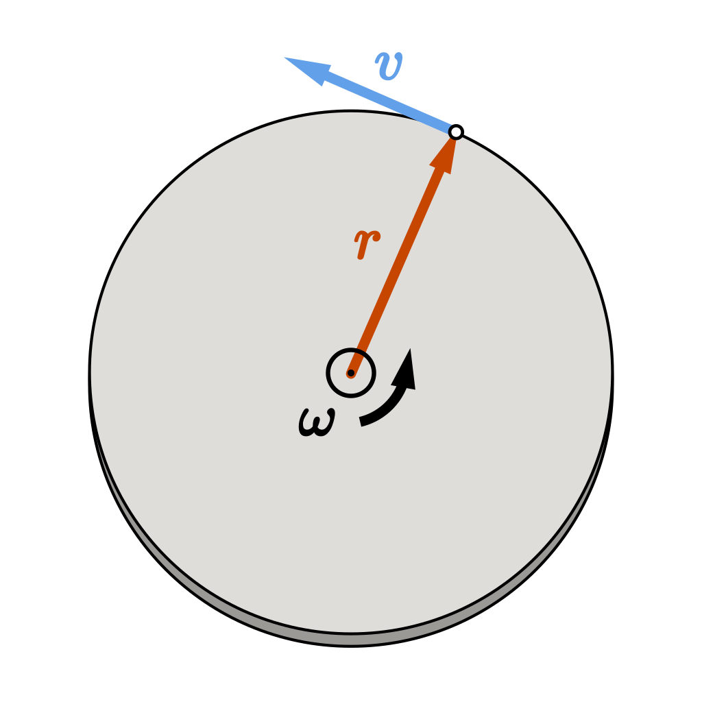
Then, the tangential (or linear) speed, is a scalar, denoted by \[v\] (or \[v_{\theta}\] when I use it to represent a signed scalar), is the component of the velocity that is along the tangent to the circular path. It is calculated by \[v=r\omega\]. This is the term that we usually use in problems where we just deal with the size of the velocity.
We call it tangential as the velocity is always directed along the tangent to the path of the object, i.e. it changes direction continuously so that the motion is always perpendicular to the radius of the circle at any given point.
In simple problems we only care about the tangential speed, \[v\], and we do not require vector \[\vec{v}\], thus the directional component, \[\hat{\theta}\] is usually ignored as it always points tangentially to the circle at the object's current position.
Though remember the full velocity is always \[v\cdot \hat{\theta}\] but if we're only discussing how fast the particle moves, we just refer to \[v\] for simplicity.
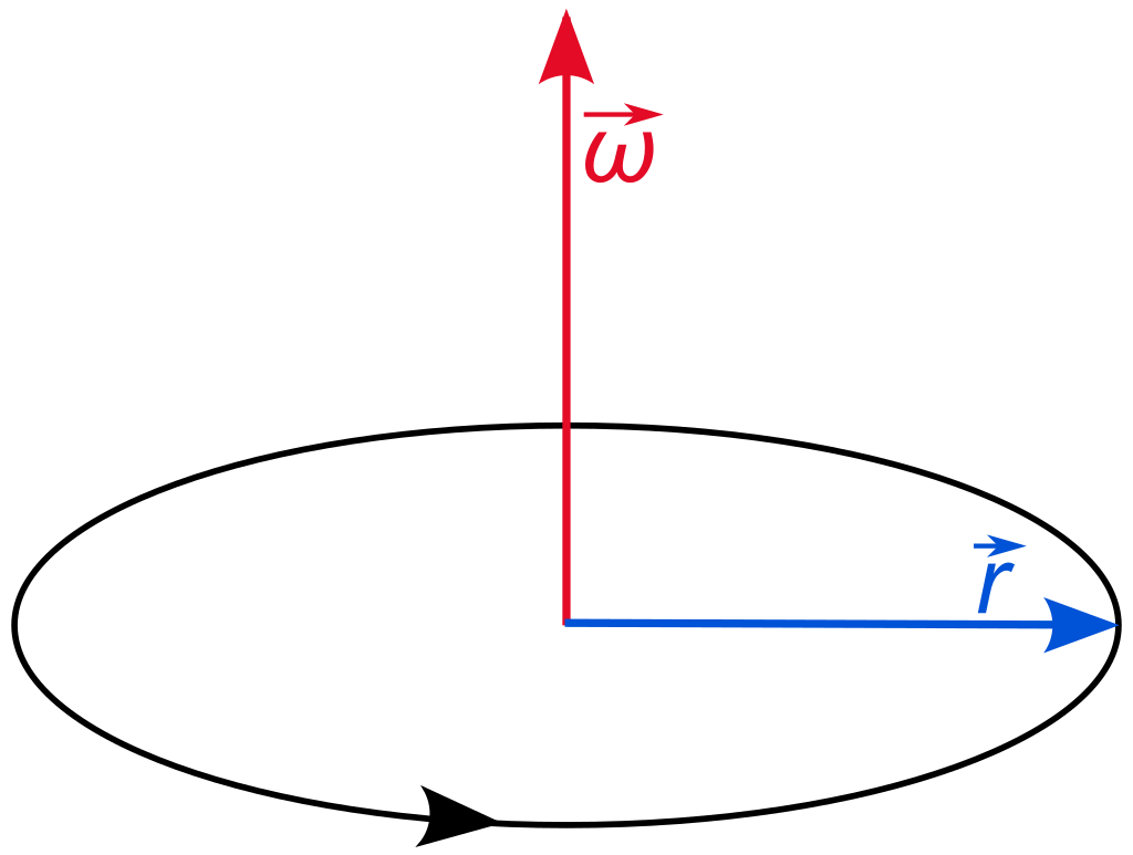
Angular velocity, usually denoted by \[\vec{\omega}\], is a pseudovector representation of how quickly an object rotates around an axis of rotation and how fast the axis itself changes direction. It usually has a direction that, by convention, is perpendicular to the plane of rotation. Again, it is comprised of the magnitude and directional component, i.e. \[\vec{\omega}=\omega\cdot\hat{n}\] where \[\hat{n}\] is the unit vector perpendicular to the plane of rotation.
Similarly, angular speed, denoted as \[\omega\] is simply the magnitude of the angular velocity (without direction). It tells you how fast the angle is changing regardless of the direction of rotation. It is calculated by \[\omega=\left| \frac{d\theta}{dt} \right|\].
You can imagine this as a spinning wheel, \[\omega\] tells us how quickly the wheel is spinning and the unit vector \[\hat{n}\] tells us the direction of the axle of the spinning wheel. When you multiply the two, you get a complete picture: the speed of rotation and the orientation of the rotation.
Again, for most cases we're only interested in how fast the angle is changing, so only we take the magnitude \[\omega\]. Typically motion is in the \[xy\]-plane and \[\hat{n}\] usually stays constant, pointing in the \[z\]-direction, which does not concern us, so for simplicity's sake we do not explicitly write that in calculations.
Derivation
We begin our description of circular motion by using polar coordinates and sketching the position vector \[\vec{r}(t)\] of the object moving in a circular orbit of radius \[r\].
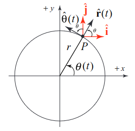
At time \[t\], the particle will be at position \[(r,\theta(t))\], call it point \[P\], and the position vector given by \[\vec{r}(t)=r\cdot\hat{r}(t)\]. Think of \[\vec{r}\] as a complete picture of the particle's position in space, i.e. how far it is and in what direction. While \[\hat{r}\] simply tells us the direction in which the particle is located relative to the center which simplifies calculations.
At point \[P\] consider two sets of unit vectors, \[(\hat{r}(t),\hat{\theta}(t))\] and \[(\hat{\imath},\hat{\jmath})\] as shown in the figure above. The vector decomposition for \[\hat{r}(t)\] and \[\hat{\theta}(t)\] in terms of \[\hat{\imath}\] and \[\hat{\jmath}\] is given by \[\hat{r}(t)=\cos(\theta(t))\cdot \hat{\imath}+\sin(\theta(t))\cdot \hat{\jmath}\] and \[\hat{\theta}(t)=-\sin(\theta(t))\cdot \hat{\imath}+\cos(\theta(t))\cdot \hat{\jmath}\].
We will then calculate the time derivatives before moving on to the velocity,
Similarly,
The velocity vector, \[\vec{v}(t)\] is then \[\vec{v}(t)=\frac{d\vec{r}(t)}{dt}=r\cdot \frac{d\hat{r}(t)}{dt}=r \frac{d\theta(t)}{dt}\cdot\hat{\theta}(t)\], meaning the velocity vector has magnitude \[r \frac{d\theta}{dt}\] and points in the direction of \[\hat{\theta}(t)\]. Intuitively, we can think of the velocity vector as a tangent arrow at the particle's location that encapsulates the particle's instantaneous speed and the direction.
We can write the result of \[\vec{v}\] as \[\vec{v}=v_{\theta}\cdot\hat{\theta}(t)\] where \[v_{\theta}=r \frac{d\theta}{dt}\] (signed), a quantity we shall refer to as the tangential component of the velocity.
More precisely, denote the magnitude of the velocity as \[v=\left\lVert \vec{v}(t) \right\rVert=r\left| \frac{d\theta}{dt} \right|\]. The magnitude (i.e. the speed) is a scalar quantity which doesn't have a direction, therefore we take the absolute value of \[\frac{d\theta}{dt}\] as it may be negative (which we are not concerned about). Next, the angular speed, or the magnitude of the rate of change of angle, is denoted by \[\omega=\left| \frac{d\theta}{dt} \right|\]. Which makes our final equation \[v=r\omega\].
Geometric derivation
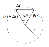
Consider a particle undergoing circular motion. At time \[t\], the particle will have a position \[\vec{r}(t)\]. After a time interval \[\Delta t\], the particle moves to the position \[\vec{r}(t+\Delta t)\]. We call this displacement \[\Delta \vec{r}\].
The magnitude of the displacement, \[\left\lVert \Delta \vec{r} \right\rVert\] can be calculated with \[\sin \frac{\Delta\theta}{2}=\frac{\frac{\left\lVert \Delta \vec{r} \right\rVert}{2}}{r}\implies \left\lVert \Delta \vec{r} \right\rVert=2r\sin \frac{\Delta\theta}{2}\].
The Taylor series expansion of \[\sin\theta=\theta-\frac{1}{6}\theta^{3}+\frac{1}{120}\theta^{5}-\cdots\], and when \[\theta\] is sufficiently small and measured in radians, only the first term of the infinite series contributes, as the successive terms in the expansion become much smaller, i.e. \[\sin\theta\approx\theta\]. This is known as small angle approximation.
Based on the above, when \[\Delta\theta\] is sufficiently small, \[\sin \frac{\Delta\theta}{2}\approx \frac{\Delta\theta}{2}\]. Then, \[\left\lVert \Delta \vec{r} \right\rVert=2r \frac{\Delta\theta}{2}=r\Delta\theta\]. Intuitively, when \[\Delta\theta\to0\], the length of the chord becomes approximately equal to the arc length, i.e. \[s=r\cdot\Delta\theta\].
The magnitude of the tangential velocity \[v\], is proportional to the rate of change of angle with respect to time, \[v=\left\lVert \vec{v}(t) \right\rVert=\lim_{\Delta t\to0}\frac{\left\lVert \Delta \vec{r} \right\rVert}{\Delta t}=\lim_{\Delta t\to0}\frac{r \left| \Delta\theta \right|}{\Delta t}=r\lim_{\Delta t\to0}\frac{\left| \Delta\theta \right|}{\Delta t}=r \left| \frac{d\theta}{dt} \right|\], which when we substitute \[\omega=\left| \frac{d\theta}{dt} \right|\], we get our equation \[v=r\omega\].