polar coordinates
Polar coordinates
Polar coordinates is a two-dimensional coordinate system in which each point on a plane is determined by a distance from a reference point and an angle from a reference direction. In simple words, a point in a plane is described as \[(r,\theta)\], where \[r\] is the distance from the origin and \[\theta\] is the angle in radians formed with the positive x-axis (usually). Instead of writing a function as \[y=f(x)\], functions are written as \[r=f(\theta)\].
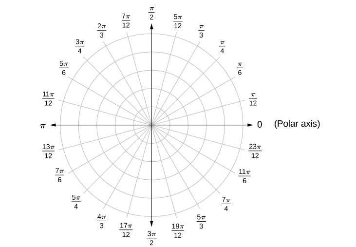
We usually plot polar coordinates in this manner,
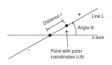
\[\theta\] will be positive anti-clockwise while negative if clockwise, similar to trigonometric calculation. On the other hand, we allow \[r\] be negative, such that \[\left( -r,\theta \right)=\left( r,\theta+\pi \right)\], which implies that there are an infinite number of coordinates for a given point. For instance, the points \[\left( 5,\frac{\pi}{3} \right)=\left( 5,-\frac{5\pi}{3} \right)=\left( -5,\frac{4\pi}{3} \right)=\left( -5,-\frac{2\pi}{3} \right)\] are all polar coordinates for the same point.
This is a consequence of the identities \[-\cos\theta=\cos(\theta+\pi)\] and \[-\sin\theta=\sin(\theta+\pi)\].
Relationship between Cartesian and polar coordinates
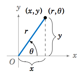
From the diagram above, we can say that \[x=r\cos\theta\] and \[y=r\sin\theta\], therefore \[x^{2}+y^{2}=r^{2}(\cos^{2}\theta+\sin^{2}\theta)=r^{2}\].
Then, \[\tan\theta=\frac{y}{x}\].
If we take the square root \[r\], we get \[\pm\sqrt{x^{2}+y^{2}}\]. To determine whether we're supposed to take the positive or negative, if we know that \[\cos\theta<0\] but \[x>0\], then it follows that \[r\] must be \[-\sqrt{x^{2}+y^{2}}\] for \[x=r\cos\theta\] to hold true. The same logic can be applied to other scenarios, e.g. \[\cos\theta>0\], \[x<0\].
However, we usually just stick with positive \[r\] and change the angle accordingly.
Distance between coordinates using law of cosines
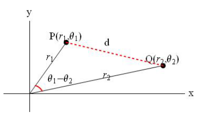
By the law of cosines, \[d^{2}=r_{1}^{2}+r_{2}^{2}-2r_{1}r_{2}\cos \left( \theta_{1}-\theta_{2} \right)\].
Graping polar functions
Polar functions are usually specified as \[r=f(\theta)\]. As an example, let \[r=\sqrt{\theta}\] and \[0\le\theta\le 2\pi\].
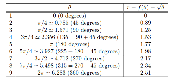
Then we plot the points,
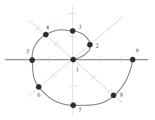
it is also to keep in mind that when we're connecting the dots, it will always be curved and never a straight line as a radial straight line implies that there are multiple \[r\] values for each \[\theta\], which goes against the definition of a function.
Now consider \[r=\frac{1}{2}+\cos\theta\].
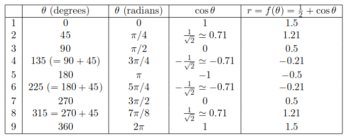
Notice that we have negative numbers for \[r\], so to graph those, we'll use the fact that \[(-r,\theta)=(r,\theta+\pi)\],
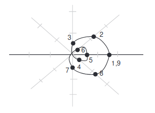
Similarly, for functions such as \[r^{2}=1+\cos\theta\implies r=\pm\sqrt{1+\cos\theta}\] (don't forget the \[\pm\]).
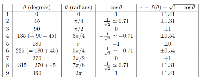
We label the positive points as \[1,2,\dots,9\] and the negative points as \[1^{\prime},2^{\prime},\dots,9^{\prime}\], then using \[(-r,\theta)=(r,\theta+\pi)\],
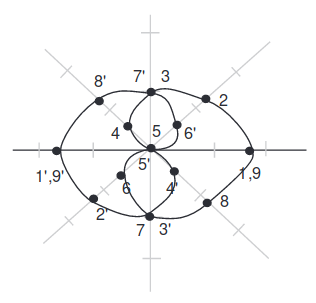
However, for odd powers like \[r^{3}\] or \[r^{5}\], we do not have to add the \[\pm\].
Area in polar coordinates
We'll start with the fact that the area of a slice of circle that has angle \[\theta\] and radius \[r\] is calculated by \[\frac{\theta}{2\pi}\cdot \pi r^{2}=\frac{1}{2}r^{2}\theta\], as a slice would be a fraction \[\frac{\theta}{2\pi}\] of the entire circle.
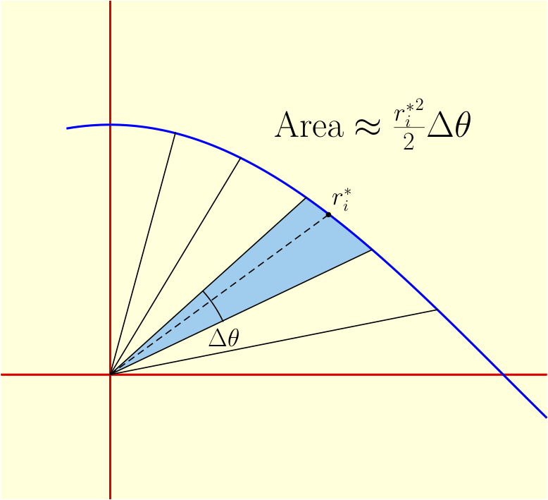
To compute the area inside of a polar curve \[r=f(\theta)\] between angles \[\theta=a\] and \[\theta=b\], we chop it into tiny pieces of angle \[\Delta\theta=\frac{(b-a)}{n}\]. These pieces have slightly different sides (due to varying \[r\]), which ultimately makes little difference when \[n\to\infty\].
Then, each \[i\]th piece has an area of approximately \[\frac{1}{2}f(\theta^{\ast}_{i})^{2}\cdot \Delta\theta\], where \[\theta_{i}^{\ast}\] is a representative angle between \[a+(i-1)\Delta\theta\] and \[a+i\Delta\theta\], so the whole thing has an area of approximately \[\sum_{i=1}^{n}\left[ \frac{1}{2}f(\theta_{i}^{\ast})^{2}\Delta\theta \right]\]. Taking the limit \[n\to\infty\] fulfills the definition of the integral, \[\int_{a}^{b}\left[ \frac{1}{2}f(\theta)^{2} \right]d\theta\implies \frac{1}{2}\int_{a}^{b}f(\theta)^{2}d\theta\].
Slopes
When we describe a curve using polar coordinates, it is still a curve in the \[x\]-\[y\] plane. First note that \[x(\theta)=f(\theta)\cos\theta\] and \[y(\theta)=f(\theta)\sin\theta\]. Then, define \[\theta(x)\] and \[\theta(y)\] as the inverse of \[x(\theta)\] and \[y(\theta)\] respectively. By the definition of functions, it follows that \[x(\theta(x))=x\] and \[y(\theta(y))=y\].
Differentiating both \[x(\theta(x))=x\] and \[y(\theta(y))=y\] with the chain rule will yield us,
Since we've defined a function of \[\theta\] in terms of \[x\], then we can define \[y(\theta(x))\] to force \[y\] to be an explicit function of \[x\]. Then,
Now, based on the derivatives of trigonometric functions and product rule, \[x^{\prime}(\theta)=f^{\prime}(\theta)\cos\theta+(-f(\theta)\sin\theta)\] and \[y^{\prime}(\theta)=f^{\prime}(\theta)\sin\theta+f(\theta)\cos\theta\]. We've defined \[y\] is in terms of \[x\], then we can conclude that \[\frac{d}{dx}[y(\theta(x))]=\frac{dy}{dx}=\frac{f^{\prime}(\theta)\sin\theta+f(\theta)\cos\theta}{f^{\prime}(\theta)\cos\theta-f(\theta)\sin\theta}\].