probability distribution

Let \[(\Omega,\mathcal{F},P)\] be a probability space and \[X(\omega)\] an \[\mathbb{R}\]-valued random variable on this space. The set function \[Q(\mathcal{B})\], defined as \[P(\omega\in \Omega:X(\omega)\in \mathcal{B})\], where \[\mathcal{B}\] is a Borel set, is called the distribution of \[X\].

In plain words, the distribution tells us the probability that \[X\] takes on a value in any subset of \[\mathbb{R}\].

If it so happens that \[Q(\mathcal{B})=\int_{A}f(x)\,dx\] then \[f\] is a density function for \[Q\], usually however, we call it the probability density function (also known as continuous probability functions) of \[X\]. Similarly, if it also happens that \[Q(\mathcal{B})\] can be written as \[\sum_{i\in A\cap \left\{ \dots,-1,0,1,\dots \right\}}f(i)\], we usually call it the probability mass function (also known as discrete probability functions).

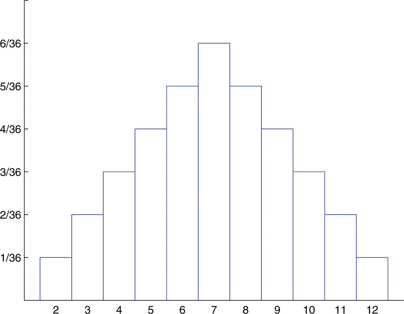
Probability distribution for tossing two fair (six-sided) dice

Informally, a discrete probability function, \[p(x)\] is a function that satisfies the following properties:

• \[P(X=x)=p(x)=p_{x}\]
  
• \[p(x)\ge0\] for all \[x\in \mathbb{R}\]
  
• The sum of \[p(x)\] over all possible values of \[x\] is 1, i.e. \[\sum_{i}p_{i}=1\], where \[i\] represents all possible values that \[x\] can have and \[p_{i}\] is the probability at \[x_{i}\]
  

Essentially, a discrete probability function is a function that can take a discrete number of values (not necessarily finite). This is most often the non-negative integers or some subset of the non-negative integers. There is no mathematical restriction that discrete probability functions only be defined at integers, but in practice this is usually what makes sense. For example, if you toss a coin 6 times, you can get 2 heads or 3 heads but not 2 and a half heads. Each of the discrete values has a certain probability of occurrence that is between zero and one. That is, a discrete function that allows negative values or values greater than one is not a probability function.

The motivation behind continuous distributions is that, not everything comes in discrete quantities. For instance, the temperature inside a room takes on a continuous set of values. One might think, well, we can also plot this out like discrete variables. Now imagine someone asks, what is the probability that the temperature at noon tomorrow will be 28 degrees Celsius? The answer would simply be zero. There is no chance that the temperature at a specific time will be exactly 28 degrees Celsius. It might be 28.01, or 28.000000001, there is an infinite number of possibilities. Thus, the probability of a very specific value occurring is \[\frac{1}{\infty}=0\].

When encountered in practice, continuous probability distributions are not only continuous, but also absolute continuous. When a random variable takes values from a continuum then by convention, any individual outcome it assigned probability zero. For such continuous random variables, only events that include infinitely many outcomes such as intervals have probability greater than zero.

A continuous probability distribution can be described by means of a cumulative distribution function, which describes the probability that the random variable is no larger than a given value, i.e. \[P(X\le x)\] for some \[x\]. The cumulative distribution function is the area under the probability density function from \[-\infty\] to \[x\].

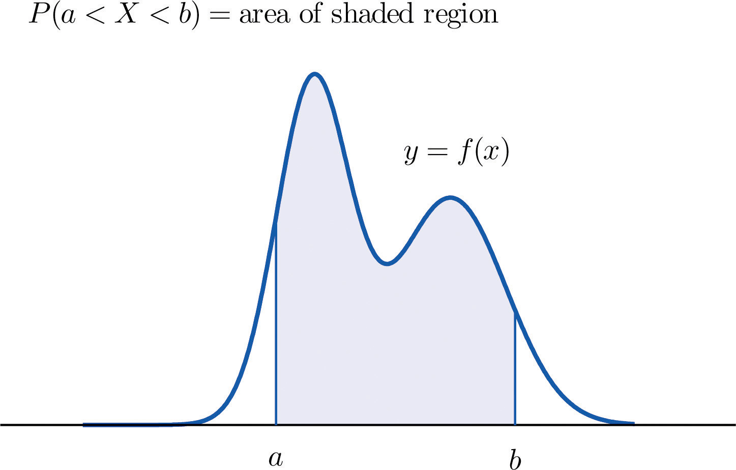
Informally, the mathematical definition of a continuous probability function, \[f(x)\], is a function that satisfies the following properties:

• The probability that \[x\] is between two points \[a\] and \[b\] is \[p(a\le x\le b)=\int_{a}^{b}f(x)\,dx\]
  
• \[f(x)\] is non-negative for \[x\in \mathbb{R}\]
  
• \[\int_{-\infty}^{\infty}f(x)\,dx=1\], note that since this is the only requirement, unlike discrete probability distributions, technically we could have a tiny interval (not wider than one unit) where \[f(x)>1\]
  

Since continuous probability functions are defined for an infinite number of points over a continuous interval, the probability at a single point is always zero. Probabilities are measured over intervals, not single points. That is, the area under the curve between two distinct points defines the probability for that interval. This means that the height of the probability function can in fact be greater than one. The property that the integral must equal one is equivalent to the property for discrete distributions that the sum of all the probabilities must equal one.