transformation matrix
Transformation matrix
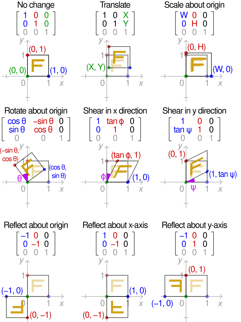
Linear transformations can be represented by matrices. If \[T\] is a linear transformation mapping \[\mathbb{R}^{n}\to \mathbb{R}^{m}\] and \[\mathbf{x}\] is a column vector with \[n\] entries, then there exists an \[m\times n\] matrix \[A\] known as the transformation matrix of \[T\], such that \[T(\mathbf{x})=A\mathbf{x}\].
Most common geometric transformations that keep the origin fixed are linear, including rotation, scaling, shearing, reflection, and orthogonal projection. In two dimensions, linear transformations can be represented using a \[2\times 2\] transformation matrix.
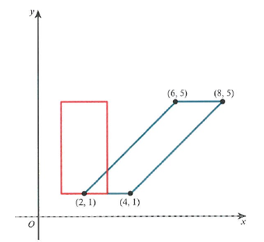
Consider a rectangle of two dimensions, \[(1,1)\], \[(1,3)\], \[(5,3)\], \[(5,1)\], we will use a matrix to represent it,
Stretching
Let's we multiply \[A\] by \[\begin{pmatrix}1 & 0 \\ 0 & 2 \end{pmatrix}\], we would get \[\begin{pmatrix}1 & 1 & 5 & 5 \\ 2 & 6 & 6 & 2\end{pmatrix}\], which would mean that each y-coordinate has been increased by a factor of 2. The new rectangle would have its length increased by a factor of 2, and it's distance from the x-axis would also be increased by a factor of 2.
Same goes with if we multiply \[A\] by \[\begin{pmatrix}2 & 0 \\ 0 & 1\end{pmatrix}\], we would get \[\begin{pmatrix}2 & 2 & 10 & 10\\ 1 & 3 & 3 & 1\end{pmatrix}\]. The new rectangle would have twice it's original width and twice as far from the y-axis as the original rectangle.
Similarly, for three-dimensional vectors, \[\begin{pmatrix}2&0&0\\0&3&0\\0&0&4\end{pmatrix}\] would equate to stretching in the x-axis by a scale factor of 2, y-axis by a scale factor of 3 and z-axis by a scale factor of 4.
Enlargement
If we multiply \[A\] by \[\begin{pmatrix}2 & 0 \\ 0 & 2\end{pmatrix}\], we would get the effect above combined, \[\begin{pmatrix}2 & 2 & 10 & 10 \\2 & 6 & 6 & 2\end{pmatrix}\], which would be a new rectangle of twice the width and length, and twice the distance from both the x-axis and the y-axis.
Reflection
If \[A\] is multiplied by \[\begin{pmatrix}-1 & 0 \\ 0 & 1\end{pmatrix}\], we would get \[\begin{pmatrix}-1 & -1 & -5 & -5 \\ 1 & 3 & 3 & 1\end{pmatrix}\], which would reflect the rectangle along the y-axis.
For three-dimensional vectors, reflections are considered as planes (two-dimensional flat surface that extends indefinitely).
Reflection on line \[y=x\]
To reflect \[A\] on the line \[y=x\], we simply multiply \[A\] by \[\begin{pmatrix} 0&1\\1&0 \end{pmatrix}\]. To understand why, look at this equation \[\begin{pmatrix} 0&1\\1&0 \end{pmatrix}\begin{pmatrix} x\\y \end{pmatrix}=\begin{pmatrix} y\\x \end{pmatrix}\].
Rotation
Assume we have a point \[x\], lying on the x-axis as such:
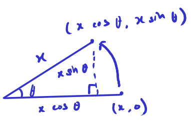
When we rotate \[x\] by \[\theta\] degrees anticlockwise, \[x\] would be at position \[(x\cos\theta,\,x\sin\theta)\], which can be proved by using the unit circle.
Applying the matrix \[B=\begin{pmatrix}a&b\\c&d\end{pmatrix}\] so that, \[B\]'s purpose here is similar to the matrix \[\begin{pmatrix}1 & 0 \\ 0 & 2 \end{pmatrix}\], and instead of transforming four points, we are transformating one point, which is \[\begin{pmatrix}x\\0\end{pmatrix}\].
From the equation above, we can conclude, \[a=\cos\theta\] and \[c=\sin\theta\]. Since the magnitude of \[\begin{pmatrix}x\\0\end{pmatrix}\] doesn't change after the transformation, \[\det(B)\] must be 1. From here, we can form the equation \[d\cos\theta-b\sin\theta=1\]. Comparing it to the equation \[\cos^{2}\theta+\sin^{2}\theta=1\], we get \[d=\cos\theta\] and \[b=-\sin\theta\].
Combining all our results,
which tells us if we apply matrix \[B\] on a point, it will transform into \[\begin{pmatrix} \cos\theta&-\sin\theta\\\sin\theta&\cos\theta \end{pmatrix}\begin{pmatrix} x\\y \end{pmatrix}=\begin{pmatrix} x\cos\theta-y\sin\theta\\x\sin\theta+y\cos\theta \end{pmatrix}\].
The reason why when we're rotating the \[x\]-coordinate from one point to the other, we're taking \[x^{\prime}=x\cos\theta-y\sin\theta\], is that if we imagine the original points \[(x,y)\] as polar coordinates, \[x=r\cos\phi,y=r\sin\phi\], when we rotate the point by an angle \[\theta\], \[x^{\prime}=r\cos(\phi+\theta)\], and substituting the cosine double-angle identity, we get \[x^{\prime}=r(\cos\phi\cos\theta-\sin\phi\sin\theta)\], subtituting back our \[x\] and \[y\] we get \[x^{\prime}=x\cos\theta-y\sin\theta\]. The similar can be shown for \[y^{\prime}\].
For a three-dimensional matrix, when we rotate it on one axis, the coordinates of the other two axis will be altered. Visual representation:
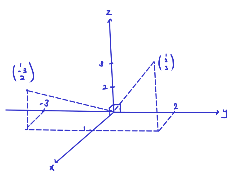
Here, we rotate the point at the x-axis, therefore the x-coordinate is unchanged, while the y and z-coordinate is altered. Therefore,
If we rotate it by the y-axis or the z-axis, the formula will be similarly as
or
Shearing
Consider a matrix \[\begin{pmatrix}1 & 1\\ 0&1\end{pmatrix}\], this would result in \[A\] having it's upper row changing to \[ax+by\], where \[a,b\] are from the matrix \[\begin{pmatrix}1 & 1\\ 0&1\end{pmatrix}\], while \[x,y\] are coordinates of a single point from matrix \[A\]. Essentially, we can simply view shearing as \[\begin{pmatrix} 1&0\\2&1 \end{pmatrix}\begin{pmatrix} x\\y \end{pmatrix}=\begin{pmatrix} x\\2x+y \end{pmatrix}\].
Visual representation: