Riemann sums
Riemann sum
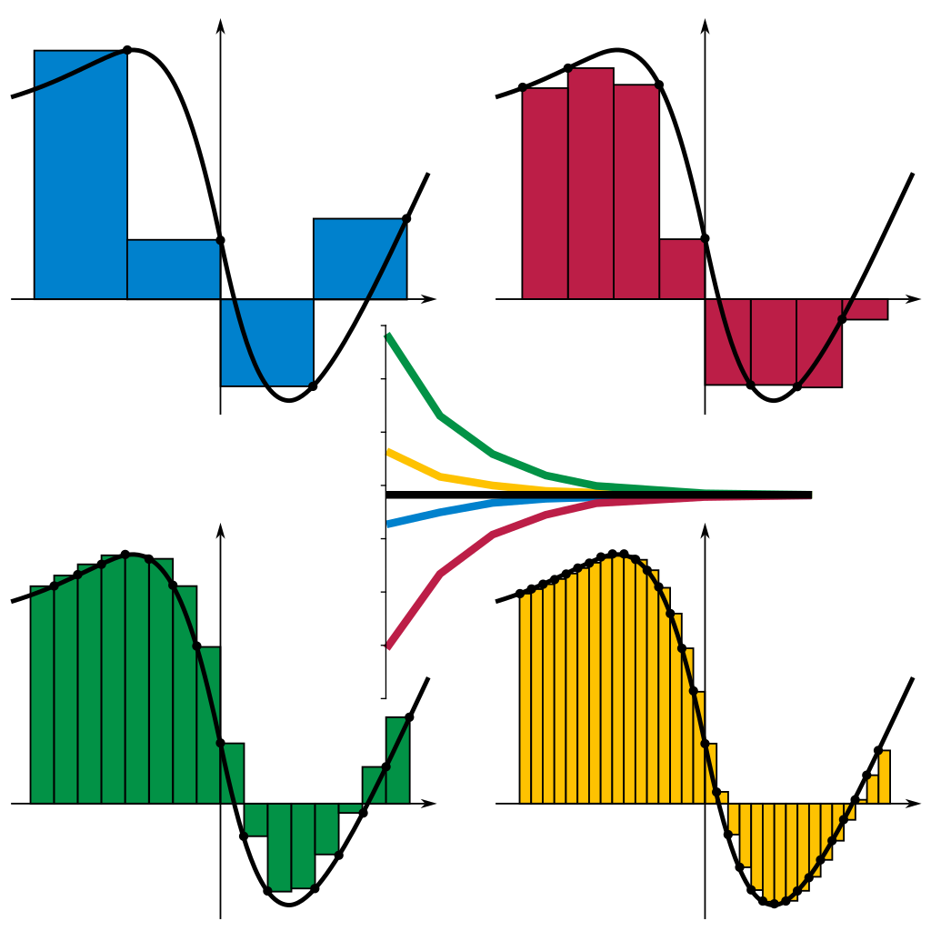
A Riemann sum is a technique used to estimate the Riemann integral, or the area under a curve, by breaking it down into smaller, manageable shapes like rectangles, trapezoids, or parabolas. This method, vital in numerical integration, involves partitioning the curve's region into sections defined by points on the x-axis. For each section, a shape that closely approximates the area underneath the curve is selected, the simplest being rectangles where height is the function's value at a specific point within the section. The areas of these shapes are calculated and then summed up to approximate the total area under the curve. Thus, the smaller these sections, the closer the sum approaches the actual integral.
Formal definition
Let \[f:[a,b]\to\mathbb{R}\] (\[[a,b]\] is the domain of the function \[f\], and \[f\in\mathbb{R}\]), and \[P=\{x_{0},x_{1},x_{2},\dots,x_{n}\}\], that is \[a=x_{0}<x_{1}<x_{2}<\cdots<x_{n}=b\]. A Riemann sum, defined as \[S\] of \[f\] over \[[a,b]\] is defined as \[S=\sum_{i=1}^{n}f(x_{i}^{\ast})\Delta x_{i}\], where \[x_{i}^{\ast}\] represents the type of Riemann sum and \[\Delta x_{i}\] is defined as \[\Delta x_{i}=x_{i}-x_{i-1}\] (width of interval \[\left[ x_{i-1},x_{i} \right]\]). However, it does not really matter what kind of \[x_{i}^{\ast}\] is chosen if \[f\] is Riemann integrable as \[\Delta x_{i}\] will approach zero anyway.
Riemann sums
Riemann sums (different from the summation methods) refer to the different types of sample points that are usually chosen in each subinterval to estimate the area under the curve.
- Left Riemann sum: \[x_{i}^{\ast}=x_{i-1}\] for all \[i\]
- Right Riemann sum: \[x_{i}^{\ast}=x_{i}\] for all \[i\]
- Middle Riemann sum: \[x_{i}^{\ast}=\frac{\left( x_{i}+x_{i-1} \right)}{2}\] for all \[i\]
- Upper Riemann sum: \[f(x_{i}^{\ast})=\sup_{x\in\left[ x_{i-1},x_{i} \right]}f(x)\]
- Lower Riemann sum: \[f(x_{i}^{\ast})=\inf_{x\in \left[ x_{i-1},x_{i} \right]}f(x)\]
Riemann summation methods
Riemann summation methods include both the choice of sample points and the overall strategy for approximating integrals.
For the sake of convenience, we assume we're integrating over the interval \[\left[ a,b \right]\] and the width of each subinterval (\[\Delta x=\frac{b-a}{n}\]) is equal.
Left Riemann sum
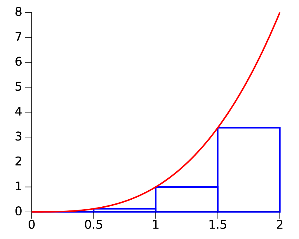
The area under the graph is approximated by drawing rectangles with heights based on the left endpoints of each subinterval, i.e. each rectangle has an area of \[\Delta x\cdot f(a+i\Delta x)\], where \[i\in \left\{ 0,1,2,\dots,n-1 \right\}\].
\[\therefore S_{\text{left}}=\sum_{i=0}^{n-1}f(a+i\Delta x)\Delta x\]
Right Riemann sum
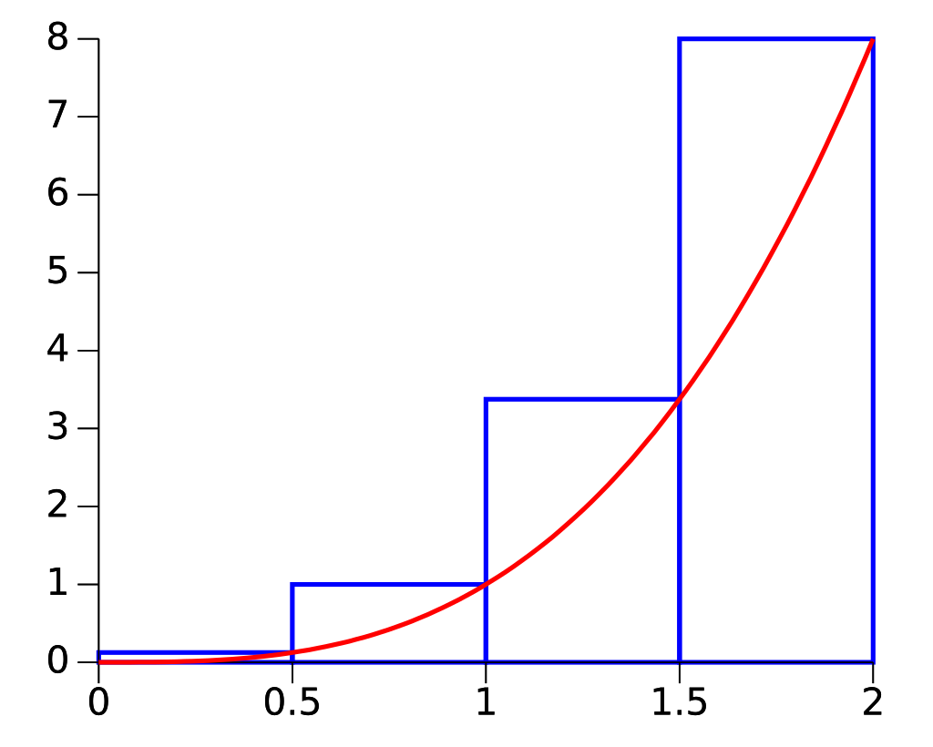
The area is approximated by drawing rectangles with heights based on the right endpoints of each subinterval, i.e. each rectangle has an area of \[\Delta x\cdot f(a+i\Delta x)\] where \[i\in \left\{ 1,2,3,\dots,n \right\}\].
\[\therefore S_{\text{right}}=\sum_{i=1}^{n}f(a+i\Delta x)\Delta x\]
Middle Riemann sum
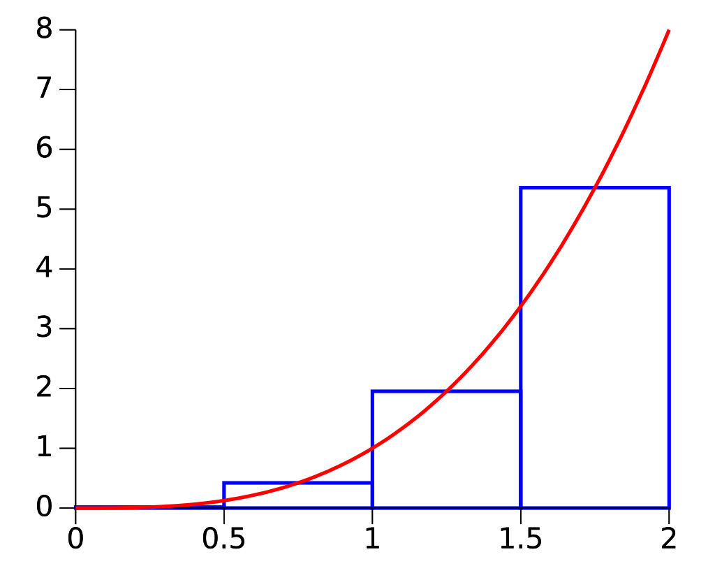
The area is approximated by drawing rectangles with heights based on the midpoints of each subinterval, i.e. each rectangle has an area of \[\Delta x\cdot f\left(a+i \frac{\Delta x}{2} \right)\] where \[i\in \left\{ 1,2,3,\dots,n \right\}\].
\[\therefore S_{\text{mid}}=\sum_{i=1}^{n}f\left(a+i \frac{\Delta x}{2} \right)\Delta x\]
Example
Calculate the area under the curve \[f(x)=x^{2}\] over \[\left[ 0,2 \right]\].
First, we define the length of each interval as \[\Delta x=\frac{2-0}{n}=\frac{2}{n}\]. We'll be using the right Riemann sum to compute the area.
Our result agrees with the integral \[\int_{0}^{2}x^{2}\,dx=\left[ \frac{x^{3}}{3} \right]^{2}_{0}=\frac{8}{3}\].