integration by parts

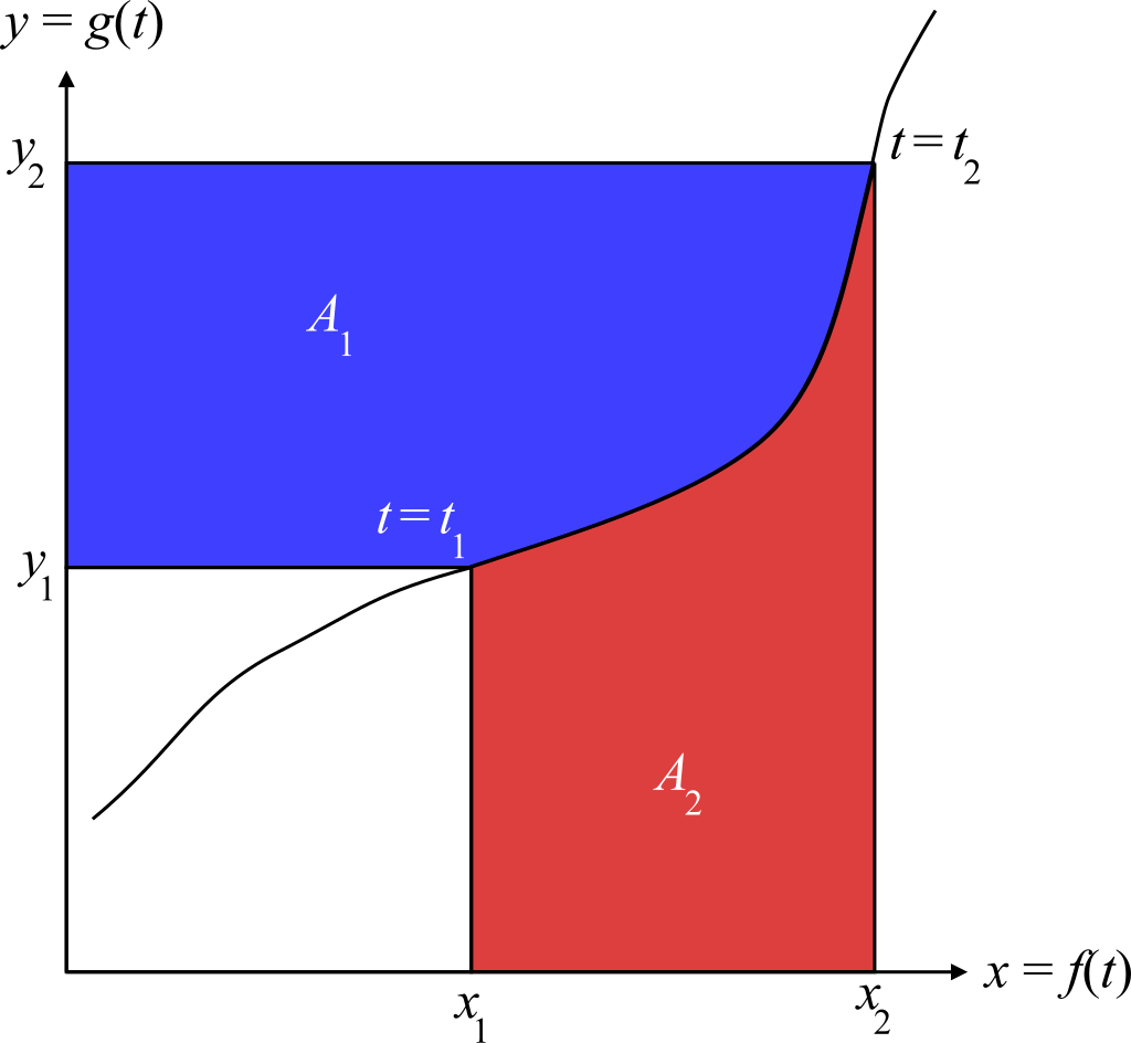
Integration by parts may be thought of as deriving the area of the blue region (\[A_{1}\]) by subtracting the smaller rectangle \[x_{1}y_{1}\] and \[A_{2}\] from the larger rectangle \[x_{2}y_{2}\].

Consider a parametric curve \[\left( x,y \right)=\left( f(t),g(t) \right)\]. We can then define \[x(y)=f(g^{-1}(y)),y(x)=g(f^{-1}(x))\], which can be derived by:

\begin{align*} y&=g(t)\implies t=g^{-1}(y)\\ x&=f(t)=f(g^{-1}(y))\\ \end{align*}

Then define \[x(y)=f(g^{-1}(y))\] which explicitly states that for \[x\] is a function of \[y\]. The similar can be shown for \[y(x)=g(f^{-1}(x))\].

The areas can then be defined as \[A_{1}=\int_{y_{1}}^{y_{2}}x(y)\,dy,A_{2}=\int_{x_{1}}^{x_{2}}y(x)\,dx\] and \[A_{1}+A_{2}=\biggl[ x\cdot y(x) \biggr]_{x_{1}}^{x_{2}}=\biggl[ y\cdot x(y) \biggr]_{y_{1}}^{y_{2}}\].

The equality \[\biggl[ x\cdot y(x) \biggr]_{x_{1}}^{x_{2}}=x_{2}y_{2}-x_{1}y_{1}\] can then be derived via,

\begin{align*} \biggl[ x\cdot y(x) \biggr]_{x_{1}}^{x_{2}}&=x_{2}\cdot y(x_{2})-x_{1}\cdot y(x_{1})\\ &=x_{2}\cdot g(f^{-1}(x_{2}))-x_{1}\cdot g(f^{-1}(x_{1}))\\ &=x_{2}\cdot g(t_{2})-x_{1}\cdot g(t_{1})\\ &=x_{2}\cdot y_{2}-x_{1}\cdot y_{1} \end{align*}

To write the formula in terms of \[t\], since \[(x,y)=(x(t),y(t))\] (meaning \[x\] and \[y\] are functions of \[t\]), then \[dy=\frac{dy}{dt}dt\] and \[dx=\frac{dx}{dt}dt\]. Additionally, \[y(t_{1})=y_{1}\], \[x(t_{2})=t_{2}\], etc., therefore,

\begin{align*} \int_{y_{1}}^{y_{2}}x(y)\,dy+\int_{x_{1}}^{x_{2}}y(x)\,dx&=\int_{t_{1}}^{t_{2}}x(t)\cdot \frac{dy}{dt}dt+\int_{t_{1}}^{t_{2}}y(t)\cdot \frac{dx}{dt}dt\\ &=\int_{t_{1}}^{t_{2}}x(t)y^{\prime}(t)\,dt+\int_{t_{1}}^{t_{2}}y(t)x^{\prime}(t)\,dt\\ \end{align*}

Notice that we can combine it to form \[\int_{t_{1}}^{t_{2}}[x(t)y^{\prime}(t)+y(t)x^{\prime}(t)]\,dt\], which we can then use the Leibniz product rule to write \[\frac{d}{dt}(x(t)y(t))=x(t)y^{\prime}(t)+y(t)x^{\prime}(t)\].

Integrate the derivative,

\begin{align*} \int_{t_{1}}^{t_{2}}x(t)y^{\prime}(t)\,dt+\int_{t_{1}}^{t_{2}}y(t)x^{\prime}(t)\,dt&=\int_{t_{1}}^{t_{2}}\frac{d}{dt}(x(t)y(t))\,dt\\ &=\biggl[ x(t)y(t) \biggr]_{t_{1}}^{t_{2}}\\ \end{align*}

as the second fundamental theorem of calculus and the definition of antiderivative tells us that if \[F^{\prime}(t)=f(t)\] then \[\int_{t_{1}}^{t_{2}}f(t)=\biggl[ F(t) \biggr]_{t_{1}}^{t_{2}}\].

Which produces the formula, \[\int_{t_{1}}^{t_{2}}x(t)y^{\prime}(t)\,dt+\int_{t_{1}}^{t_{2}}y(t)x^{\prime}(t)\,dt=\biggl[ x(t)y(t) \biggr]_{t_{1}}^{t_{2}}\], or \[\int_{t_{1}}^{t_{2}}x(t)y^{\prime}(t)\,dt=\biggl[ x(t)y(t) \biggr]_{t_{1}}^{t_{2}}-\int_{t_{1}}^{t_{2}}y(t)x^{\prime}(t)\,dt\].

When rewritten into the indefinite integral form, we get \[\int x(t)y^{\prime}(t)\,dt=x(t)y(t)-\int y(t)x^{\prime}(t)\,dt\] (we usually omit the \[C\] when writing the formula as it is an arbitrary constant).

The integration by parts formula states: \[\int u(x)v^{\prime}(x)\,dx=u(x)v(x)-\int u^{\prime}(x)v(x)\,dx\].

This theorem can be derived using the product rule. Let \[u(x)\] and \[v(x)\] be continuously differentiable functions.

Then, the product rule states that \[\left( u(x)v(x) \right)^{\prime}=u^{\prime}(x)v(x)+u(x)v^{\prime}(x)\]. Integrating both sides we get \[\int \left( u(x)v(x) \right)^{\prime}\,dx=\int u^{\prime}(x)v(x)\,dx+\int u(x)v^{\prime}(x)\,dx\].

Now using the definition of antiderivatives we get \[u(x)v(x)=\int u^{\prime}(x)v(x)\,dx+\int u(x)v^{\prime}(x)\,dx\] or \[\int u(x)v^{\prime}(x)\,dx=u(x)v(x)-\int u^{\prime}(x)v(x)\,dx\].

If we take the integral from \[a\] to \[b\] of both sides, we get \[\int_{a}^{b} u(x)v^{\prime}(x)\,dx=\biggl[ u(x)v(x) \biggr]_{a}^{b}-\int_{a}^{b} u^{\prime}(x)v(x)\,dx\].

The LIATE rule is a rule of thumb for integration by parts. It involves choosing as \[u\] the function that comes first in the following list:

• Logarithmic functions, e.g. \[\ln(x),\log_{b}(x)\]
  
• Inverse trigonometric functions, e.g. \[\sin^{-1}(x)\]
  
• Algebraic functions, e.g. \[3x^{2}\]
  
• Trigonometric functions, e.g. \[\sin(x)\]
  
• Exponential functions, e.g. \[e^{x},19^{x}\]
  

Additionally, there are a few typical situations where we should try to use integration by parts, see here.

Evaluate \[\int_{0}^{4}xe^{-x}\,dx\].

Following the LIATE rule, let \[u(x)=x\] and \[v^{\prime}(x)=e^{-x}\]. Then, \[u^{\prime}(x)=1\] and \[v(x)=\int e^{-x}\,dx=-e^{-x}\].

\begin{align*} \int_{0}^{4}xe^{-x}\,dx&=\biggl[ -xe^{-x} \biggr]_{0}^{4}-\int_{0}^{4}1\cdot -e^{-x}\,dx\\ &=\biggl[ \left( -xe^{-x} \right)-\left( e^{-x} \right) \biggr]_{0}^{4}\\ &=\biggl[ -4e^{-4}-e^{-4} \biggr]-\biggl[ 0-e^{-0} \biggr]\\ &=-5e^{-4}+1 \end{align*}

Now, there are also cases where we have to apply the formula more than once. Evaluate \[\int\left( x-1 \right)^{3}e^{2x}\,dx\].

Again, following the LIATE rule, let \[u(x)=\left( x-1 \right)^{3}\] and \[v^{\prime}(x)=e^{2x}\]. Then, \[u^{\prime}(x)=3(x-1)^{2}\cdot 1\] and \[v(x)=\int e^{2x}\,dx=\frac{e^{2x}}{2}\].

Using the formula, we would get \[\int (x-1)^{3}e^{2x}\,dx=\left( (x-1)^{3}\cdot \frac{e^{2x}}{2} \right)-\int \left( 3(x-1)^{2}\cdot \frac{e^{2x}}{2} \right)\,dx\]. However, this is not the final answer, as we now have to solve for \[\int \left( 3(x-1)^{2}\cdot \frac{e^{2x}}{2} \right)\,dx\]. Thus, we repeat the entire process again. Let \[u(x)=3(x-1)^{2}\] and \[v^{\prime}(x)=\frac{e^{2x}}{2}\]. Then, \[u^{\prime}(x)=6(x-1)\cdot 1\] and \[v(x)=\int \frac{e^{2x}}{2}\,dx=\frac{e^{2x}}{4}\].

\begin{align*} \int(x-1)^{3}e^{2x}\,dx&=\left( (x-1)^{3}\cdot \frac{e^{2x}}{2} \right)-\left( 3(x-1)^{2}\cdot \frac{e^{2x}}{4}- \left( \int6(x-1)\cdot \frac{e^{2x}}{4}\,dx \right) \right)\\ &=\left( (x-1)^{3}\cdot \frac{e^{2x}}{2} \right)-\left( 3(x-1)^{2}\cdot \frac{e^{2x}}{4} \right) + \left( \int6(x-1)\cdot \frac{e^{2x}}{4}\,dx \right)\\ \end{align*}

We will then recursively repeat this process for every new integral that's produced until there are no more integrals left:

\begin{align*} \int(x-1)^{3}e^{2x}\,dx&=\left( (x-1)^{3}\cdot \frac{e^{2x}}{2} \right)-\left( 3(x-1)^{2}\cdot \frac{e^{2x}}{4} \right) + \left( \int6(x-1)\cdot \frac{e^{2x}}{4}\,dx \right)\\ &=\left( (x-1)^{3}\cdot \frac{e^{2x}}{2} \right)-\left( 3(x-1)^{2}\cdot \frac{e^{2x}}{4} \right)+\left( 6(x-1)\cdot \frac{e^{2x}}{8} \right)-\left( \int6\cdot \frac{e^{2x}}{8}\,dx \right)\\ &=\left( (x-1)^{3}\cdot \frac{e^{2x}}{2} \right)-\left( 3(x-1)^{2}\cdot \frac{e^{2x}}{4} \right)+\left( 6(x-1)\cdot \frac{e^{2x}}{8} \right)-\left( 6\cdot \frac{e^{2x}}{16} \right)+\left( \int0\cdot \frac{e^{2x}}{16}\,dx \right)\\ &=(x-1)^{3}\frac{e^{2x}}{2}-3(x-1)^{2}\frac{e^{2x}}{4}+6(x-1)\frac{e^{2x}}{8}-\frac{6e^{2x}}{16}+C \end{align*}

To make this process less painful, we can draw a table as such:

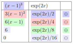
where we repeatedly differentiate the left column and integrate the right column until one of the rows get to zero.