equipartition theorem
Equipartition theorem
In classical statistical mechanics, the equipartition theorem relates the temperature of a system to its average energies. The original idea of equipartition was that, in thermal equilibrium, energy is shared equally among all of its various forms, on the average, once the system has reached thermal equilibrium; for instance, the average kinetic energy per degrees of freedom in translational motion (motion of the centre of mass) of a molecule should equal that in rotational motion.
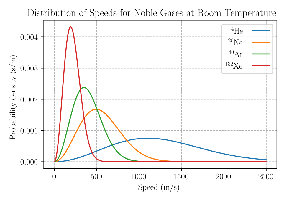
Equipartition also makes quantitative predictions for these energies. For example, it predicts that every atom of an inert noble gas, in thermal equilibrium at temperature \[T\], has an average translational kinetic energy of \[\frac{3}{2}k_{\text{B}}T\] (because it has three translational degrees of freedom, i.e. \[(x,y,z)\]), where \[k_{\text{B}}\] is the Boltzmann constant. As a consequence, since kinetic energy is equal to \[\frac{1}{2}mv^{2}\], the heavier atoms of xenon have a lower average speed than do the lighter atoms of helium at the same temperature.
Intuitive idea
The equipartition of energy theorem states that in equilibrium, each degree of freedom contributes \[\frac{1}{2}k_{\text{B}}T\] to the average energy per molecule. In other words, the internal energy of an ideal gas is \[E_{\text{internal}}=N\cdot \frac{n}{2}k_{\text{B}}T\], where \[N\] represents the number of molecules in the gas and \[n\] represents the degrees of freedom.
Notice that many of the energy terms in physics are some quadratic forms of a variable, such as \[\frac{1}{2}mv^{2}\] and \[\frac{1}{2}kx^{2}\]. This idea can be extended further, i.e. most types of energy can be expressed as a sum of quadratic terms. Assume we have a \[\ce{H-H}\] molecule. The translational kinetic energy has three terms for the three dimensions of space: \[E_{\text{tr}}=\frac{1}{2}m\dot{x}^{2}+\frac{1}{2}m\dot{y}^{2}+\frac{1}{2}m\dot{z}^{2}\], thus three degrees of freedom, \[E_{\text{tr}}\to \frac{3}{2}k_{\text{B}}T\]. It also has two perpendicular axes about which it can rotate, i.e. its angular kinetic energy is \[E_{\text{rot}}=\frac{1}{2}I\omega_{1}^{2}+\frac{1}{2}I\omega_{2}^{2}\], which corresponds to two degrees of freedom, \[E_{\text{rot}}\to\frac{2}{2}k_{\text{B}}T\]. Finally, it can have vibrational energy, which is modelled as a classical one-dimensional harmonic oscillator: \[E_{\text{vib}}=\underbrace{\frac{1}{2}m\dot{x}^{2}}_{\text{kinetic}}+\underbrace{\frac{1}{2}(m\omega^{2})x^{2}}_{\mathrm{potential}}\], \[E_{\text{vib}}\to\frac{2}{2}k_{\text{B}}T\].
However, it is to note that degrees of freedom increases with temperature. For instance, at room temperature, the internal energy of \[\ce{H2}\] gas is only \[\frac{5}{2}k_{\text{B}}T\], as it only has three translational and two rotational degrees of freedom. At temperatures well above room temperature, there are two additional vibrational degrees of freedom, thus \[E_{\text{internal}}=\frac{7}{2}k_{\text{b}}T\].
If a system can absorb energy because it is in contact with a reservoir held at temperature \[T\], where does the energy get stored? To answer this, we calculate the expectation value of the energy using Boltzmann's distribution. For a generic energy term of the form \[E=ax^{2}\], the expected value of energy \[\left\langle E \right\rangle=\frac{1}{2}k_{\text{B}}T\]. Now this reveals something surprising, \[a\] has no effect on the expectation value of \[E\]. In other words, each quadratic term contributes an energy of \[\frac{1}{2}k_{\text{B}}T\] per degree of freedom.
Derivation
Suppose the Hamiltonian of some given system has the form \[H(x,y,z,p_{x},p_{y},p_{z})=ax^{2}+K(y,z,p_{x},p_{y},p_{z})\], where \[K\] accounts for any contributions which do not involve \[x\]. In thermal equilibrium, the average value of \[ax^{2}\], i.e. the sum of \[ax^{2}\] in each possible state weighted by the probability of that state, is equal to \[\left\langle ax^{2} \right\rangle=\sum_{i}ax_{i}^{2}p_{i}=\frac{1}{Z}\sum_{i}ax_{i}^{2}e^{-\beta \left( ax_{i}^{2}+K_{i} \right)}\]. To explain further regarding the symbols, the probability \[p_{i}=\frac{e^{-\beta E_{i}}}{Z}\], where \[\beta=\frac{1}{k_{\text{B}}T}\] represents the thermodynamic beta. \[e^{-\beta E_{i}}\] is the Boltzmann factor, which indicates that lower energy states are more probable than higher energy states at thermal equilibrium. \[Z=\sum_{i}e^{-\beta E_{i}}=\sum_{i}e^{-\beta \left( ax_{i}^{2}+K_{i} \right)}\] is the canonical partition function (Zustandssumme), which serves as a normalization constant, to ensure that the sum of probabilities over all possible microstates equal to one, \[\sum_{i}p_{i}=1\].
Assume that the temperature is high enough that many terms in the sum contribute significantly, therefore it can be well approximated by an integral. Using the property that mutually orthogonal states are uniformly distributed in phase space, we find \[\left\langle ax^{2} \right\rangle=\frac{\iiint\iiint ax^{2}e^{-\beta ax^{2}}e^{-\beta K}\,dx\,dy\,dz\,dp_{x}\,dp_{y}\,dp_{z}}{\iiint\iiint e^{-\beta ax^{2}}e^{-\beta K}\,dx\,dy\,dz\,dp_{x}\,dp_{y}\,dp_{z}}\]. We can then simplify this further,
Next, we move \[a\] out form the numerator and evaluate the Gaussian integral \[\int_{-\infty}^{\infty}x^{2}e^{-\beta ax^{2}}\,dx\] using integration by parts. Let \[u=x\] and \[v^{\prime}=xe^{-\beta ax^{2}}\], then \[u^{\prime}=1\] and \[v=\int xe^{-\beta ax^{2}}\,dx\].
To solve \[v\], use integration by substitution. Recognise that we can rewrite it as \[\int e^{-\beta ax^{2}}(x\,dx)\]. Let \[f(x)=e^{x}\], \[F(x)=\int e^{x}\,dx=e^{x}\] and \[g(x)=-\beta ax^{2}\], \[g^{\prime}(x)=-2\beta ax\]. Recall that our goal is to form \[\int f(g(x))\cdot g^{\prime}(x)\,dx=F(g(x))+C\]. To achieve this, we rewrite \[v\] as \[\left( -\frac{1}{2a\beta} \right)\int e^{-\beta ax^{2}}\cdot (-2\beta ax)\,dx=\left( -\frac{1}{2a\beta} \right) \left( e^{-\beta ax^{2}}+C \right)\]. Cleaning everything up, \[v=-\frac{1}{2a\beta}e^{-\beta ax^{2}}\].
Combining the results, \[\int_{-\infty}^{\infty}(x)\left( xe^{-\beta ax^{2}} \right)\,dx=\biggl[ x\cdot\frac{1}{2a\beta}e^{-\beta ax^{2}} \biggr]_{-\infty}^{\infty}-\int_{-\infty}^{\infty}\left( 1\cdot -\frac{1}{2a\beta}e^{-\beta ax^{2}} \right)\,dx\]. To evaluate the first term, rewrite it as \[\frac{1}{2a\beta}\left( \lim_{x\to\infty}xe^{-\beta ax^{2}}-\lim_{x\to-\infty}xe^{-\beta ax^{2}} \right)\], which is already obvious that both limits will tend to zero. However, for the sake of rigour, we shall show it with l'Hôpital's rule. Let \[k=a\beta>0\], \[xe^{-\beta ax^{2}}=\frac{x}{e^{kx^{2}}}\], when \[x\to +\infty\], both numerator and denominator diverges to \[\frac{\infty}{\infty}\]. This allows us to apply l'Hôpital's rule once. Differentiate the numerator and denominator separately, \[\lim_{x\to \infty}\frac{1}{2kxe^{kx^{2}}}=0\], which proves that the whole fraction tends to zero. So, we're evaluated that \[\int_{-\infty}^{\infty}(x)\left( xe^{-\beta ax^{2}} \right)\,dx=\int_{-\infty}^{\infty}x^{2}e^{-\beta ax^{2}}\,dx=\int_{-\infty}^{\infty}\frac{1}{2a\beta}e^{-\beta ax^{2}}\,dx\].
Back to simplifying \[\frac{\int_{-\infty}^{\infty} ax^{2}e^{-\beta ax^{2}}\,dx}{\int_{-\infty}^{\infty} e^{-\beta ax^{2}}\,dx}\]. With the results that we just evaluated,