electric current
Electric current
Electric current, \[I\], is a flow of charged particles, most commonly electrons, moving through an conductor or space. It is defined as the net rate of flow of electric charge through a surface. The moving (charged) particles are sometimes called charge carriers.
Mathematically, \[I=\frac{\Delta Q}{\Delta t}\], with units ampere, where \[Q\] is the charge of each charge carrier. One can understand one \[I\] as one coulomb of charge passing through a given area per second.
The elementary (electron) charge is approximately \[e\approx1.6022\times10^{-19}\text{C}\], which implies that one coulomb of charge is equivalent to \[\frac{1}{1.6022\times10^{-19}}\approx6.2414\times10^{18}\] electrons. Thus, one can understand one \[I\] as one coulomb of charge or approximately \[6.2414\times10^{18}\] electrons passing through a given area per second.
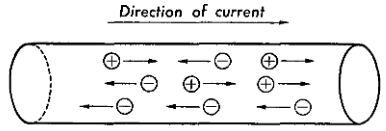
In a conductor, the flow of negative charge to the left is equivalent to a flow of positive charge to the right. Unless specifically stated, the equations dealing with electric currents are based upon the convention that the direction of the current is the direction of flow of positive charge.
Current density
When dealing with the flow of electricity in a continuous medium, it is convenient to speak of the current density, \[\mathbf{J}\]. It is defined as the quantity of charge passing through a unit area perpendicular to the direction of motion of the charge per unit time. When given the current \[I\] and area \[A\], the magnitude of \[\mathbf{J}\], is given as \[J=\frac{I}{A}\] with direction being the direction of current.
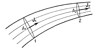
The flow of current through of a conductor of variable cross section can also be represented as somewhat of a fluid flow. Assuming the current density passing through any point in a conductor is constant, the current density in a conductor of nonuniform cross-section is inversely proportional to the cross-sectional area. That is, \[I_{1}=I_{2}\implies J_{1}\cdot A_{1}=J_{2}\cdot A_{2}\], therefore \[\frac{J_{1}}{J_{2}}=\frac{A_{2}}{A_{1}}\]. Now this analogy is useful through the use of electrolytic plotting tanks.
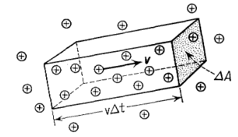
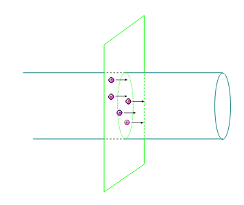
Suppose a positively charged cloud containing \[n\] particles per unit volume, each with charge \[q\] is moving with velocity \[v\]. During a short interval \[\Delta t\], every charged particle in a "slab" of space that is of base \[\Delta A\] and height \[v\Delta t\], directly upstream from a surface of area \[\Delta A\] will cross the surface and continue downstream. Then, by counting how much charge crosses per unit time and per unit area you get the current density \[J\] through that point.
First, we calculate the volume of the slab itself, \[\Delta A\cdot(v\Delta t)\], which tells us that this slab must have \[n\cdot\Delta A\cdot(v\Delta t)\] charged particles, then since each particle carries charge \[q\], this slab of particles can be said to carry \[nqv\Delta A\Delta t\] amount of charge. We've established above that \[I=\frac{Q}{\Delta t}=\frac{nqv\Delta A\Delta t}{\Delta t}=nqv\Delta A\], then \[J=\frac{I}{A}=\frac{nqv\Delta A}{\Delta A}=nqv\].