statistical hypothesis test
Statistical hypothesis test
Intuition
Suppose we have a population consisting of a thousand women (assume they are of the same age to keep it simple) in a town with varying height. Then, we are presented with a statistical hypothesis, "The average height of women in a town is 169 centimetres."
Our null hypothesis, or \[H_{0}\], would be "The population mean height is 169 centimetres". The alternate hypothesis, or \[H_{1}\] is simply the hypothesis, "The population mean height is NOT 169 centimetres." We don't know whether this is true, so we put it to the test by taking a sample of twenty women and their mean height comes to 168 centimetres. This pretty much reaffirms our hypothesis. Now, we take another sample of twenty women, and their mean height turns out to be 162 centimetres.
A question we should ask ourselves here is "how much doubt does this cast upon my hypothesis?" and "is our sample mean far enough away from 169 centimetres for us to confidently reject \[H_{0}\]?". This brings us to normal distributions and confidence intervals. The intuition is quite simple, if we have a huge enough independent samples from a population, the mean of the samples will be normally distributed. We can then convert this normal distribution into its standard normal form to ascertain how significantly our \[H_{0}\] holds and whether we want to reject or accept it.
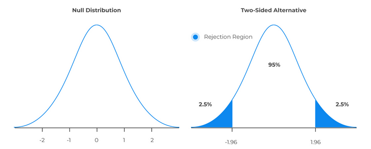
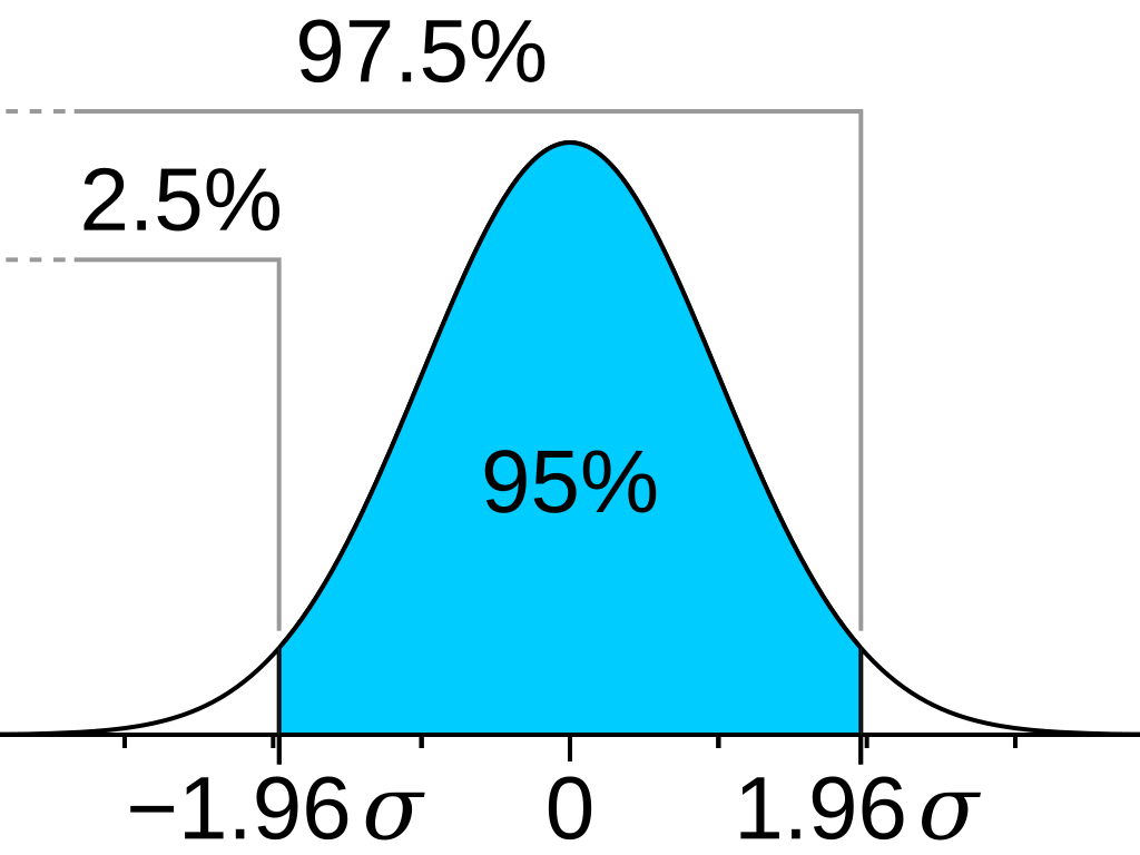
A 95 (or 90, or perhaps some other arbitrary number) percent confidence interval is usually chosen, and then we might say that there is a 95% (often written as \[0.95\]) that a given sample (normalized) mean will lie between the Z-scores \[-1.96\] and \[1.96\]. This is the concept behind the confidence interval, it provides us with the two values along with the level of confidence that our sample would lie between those values. Additionally, this means that our assumption will be correct 95 percent of the time, and in the remaining five percent of the situations, it might not hold. This is known as the significance level, or alpha \[\alpha\]. The significance level is also often represented as a decimal \[5\%\implies 0.05\]. Now, what this does is that it allows us (assuming we're taking a \[0.95\] confidence interval), to say that if a sample is within the rejection region, then we can "confidently" reject \[H_{0}\].
This method is similar to the "reductio ad absurdum" method used in logic and philosophy. We assume \[H_{0}\] to be true, then show that something ridiculous follows from that assumption and then conclude that since that happened, then \[H_{0}\] is probably false.
There is a caveat to this method as we are making decisions on the basis of the evidence that we have gathered and not a 100 percent guaranteed proof. There is always a chance to get an extreme sample which makes us reject \[H_{0}\] or \[H_{1}\]. Thus, we have coined two types of errors, type I and type II. Type I error happens when we reject \[H_{0}\] when \[H_{0}\] is true, while type II error happens when we do not reject \[H_{0}\] when it is in fact false.
Terminology
Statistical hypothesis
A statement about the parameters describing a population.
Test statistic
A test statistic assesses how consistent your sample data are with the null hypothesis in a hypothesis test. Test statistic calculations take your sample data and boil them down to a single number that quantifies how much your sample diverges from the null hypothesis. As a test statistic value becomes more extreme, it indicates larger differences between your sample data and the null hypothesis. Note that different tests have different formulas for the test statistic, but usually you'll see the sample mean or proportion converted to a \[Z\] or \[t\]-score.
Suppose the task is to test whether a coin is fair. The coin is flipped a hundred times and the results are recorded. One simple, yet sensible test statistic here is to use the number of heads, as we can use it for a variety of tests such as the binomial test.
Null hypothesis, \[H_{0}\]
\[H_{0}\], read as H-naught, is a statement about the value of a population parameter, e.g. the population mean or proportion. It can be written mathematically as, e.g. \[H_{0}:\mu=157\].
Alternate hypothesis, \[H_{1}\]
The alternate hypothesis is the claim to be tested, i.e. the opposite of \[H_{0}\]. It contains the value of the parameter that we consider plausible and is denoted as \[H_{1}\], e.g. \[H_{1}:\mu\ne 157\] or \[H_{1}:\mu>157\].
\[p\]-value
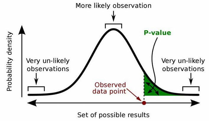
The \[p\]-value is the probability of obtaining a test results as extreme as the observed result (realization), or a more extreme result, under the assumption that \[H_{0}\] is correct. A small \[p\]-value for an observation, "small" usually being relative to the level of significance \[\alpha\], means that the probability of observing that value is "unlikely". When we say, e.g. \[p=0.03\], it is a shorthand of saying, the probability of us observing an outcome this extreme or even more extreme is \[0.03\] if our null hypothesis is correct.
Level of significance, \[\alpha\]
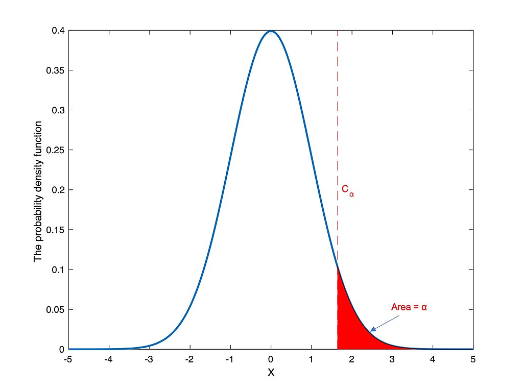
An example of the rejection region (unshaded region) in a two-tailed test, where \[\alpha=0.05\].
The level of significance, usually denoted by \[\alpha\] is the probability that the test statistic will fall into the critical region when the null hypothesis is true. Conventionally, \[\alpha\] is usually set to \[0.05\] or \[0.025\] or even \[0.001\] (if the experiment requires such an accuracy), but it can be any other value as per the discretion of whoever that is running the experiment.
Critical value
The value that defines the rejection zone, sometimes denoted by \[c\].
Assume we're testing if a person truly has clairvoyance. The procedure goes as such, we show them a back face of a random chosen playing card 25 times and ask them which of the four suits they belong to. We then record the number of correct answers and call it \[X\]. As we try to find evidence of their clairvoyance, for the time being \[H_{0}\] will be that they are not a clairvoyant. Since the probability of us picking any single suit is \[\frac{1}{4}\], then let the probability of guess it correctly be \[p\], \[H_{0}:p=\frac{1}{4}\] and \[H_{1}:p>\frac{1}{4}\].
If the person correctly guesses 20 and above, we can pretty much consider them a clairvoyant, while if they only guess 5 or 6 right, there is no cause to consider them so. Now the question is, what is the critical number, \[c\], or correct guesses, at which point we consider them to be clairvoyant? If we choose 25 correct guesses in order for them to be considered a clairvoyant, \[c=25,P \left( X=c\mid p=\frac{1}{4} \right)=\left( \frac{1}{4} \right)^{25}\approx 10^{-15}\]. This tells us that if we set the criteria to 25 correct guess, the probability of us incorrectly determining someone as a clairvoyant is \[0.\underbrace{000\dots000}_{\text{fourteen 0's}}1\], which is practically impossible. Being less critical, let's say we want our error rate to be one out of a hundred, i.e. \[c=13\], and is calculated via \[P \left( X\ge c\mid p=\frac{1}{4} \right)\le 0.01\].
Procedure
- Choose a null hypothesis \[H_{0}\] and its alternative \[H_{1}\]
- Choose a threshold \[\alpha\]
- Choose a test statistic
- Derive a distribution (the reference distribution) of the test statistic under the null hypothesis
- Compute \[p\]-value by comparing the observed value of the test statistic against its reference distribution
- Reject the null hypothesis if the \[p\]-value is less than the pre-specified threshold \[\alpha\] and retain the null hypothesis otherwise
Referenced by:
No backlinks found.